Research - (2025) Volume 20, Issue 1
Comparison of the negative exponential and weibull models for cumulative maternal mortality in red sea state, Sudan
Alshaikh A. Shokeralla*Received: 25-Jan-2025, Manuscript No. gpmp-25-161700; Editor assigned: 27-Jan-2025, Pre QC No. P-161700; Reviewed: 11-Feb-2025, QC No. Q-161700; Revised: 28-Feb-2025, Manuscript No. R-161700; Published: 31-Mar-2025
Abstract
This study was carried out to compare two growth models, namely the negative exponential model and the Weibull model, to analyze cumulative maternal mortality in the Red Sea State from 2017 to 2023. These models were compared based on goodness-of-fit statistics. The findings of this current study suggest that the Weibull model may be the most appropriate for describing the accumulation of maternal mortality in the Red Sea State. These models were evaluated using the goodness-of-fit criteria (Radj2, F-test, AIC, BIC, and AICc). According to the current study, the Weibull model is the best fitting model to characterize cumulative maternal mortality in the Red Sea State, as it has the highest Radj2 and the lowest BIC and AICc values. According to Weibull model estimates, cumulative maternal mortality in the Red Sea State will increase at a rate ranging from 17231.6 cases (95% P.I.:10904.4; 23559) to 48453.5 cases (95% P.I.:37452.7; 134360) over the next four years (2024-2025). The given fitting models and some measurements in this study were implemented using the "Nonlinear Regression" tool available in Minitab 18.1, using the nonlinear least squares method. Each model parameter's starting value was obtained using the initial value conditions and the simple linear regression equation.
Keywords
Growth models; Maternal mortality; Non-linear regression; Weibull model; Negative exponential model
Introduction
The rate of mother mortality during pregnancy, birth, and the postpartum period is an important gauge of any nation's healthcare quality. "The total cessation of all signs of life in a human being at any point following birth," the World Health Organization defines maternal death. This term especially concerns postpartum or pregnancy-related mother fatalities. Maternal mortality affects not only individual mothers but also children, families, and society, thus affecting quality of life, so impeding human, economic, and social development, and so limiting chances for growth and prosperity.
Maternal mortality continues to be a significant issue worldwide, particularly in low-income and conflict-affected regions. Research indicates that insufficient healthcare infrastructure, absence of prenatal and postnatal care, poverty, and social and cultural obstacles greatly contribute to elevated maternal death rates. In many developing nations, maternal mortality is increased when people put off getting medical help, obtaining healthcare services, and getting the right treatment [1]. Models from mathematics and statistics are used to analyses mortality patterns, forecast future instances, and create intervention strategies. In contrast to the traditional Weibull and exponential reliability models, Polito [2] proposed alternative distributions that could better capture survival and failure rates in medical settings.
The Weibull distribution is extensively used in survival analysis and reliability modelling across several disciplines, including as medicine, engineering, and epidemiology. Gupta and Kundu [3] analyzed the distinctions between the Weibull distributions and generalized exponential distributions, emphasizing the significance of selecting a suitable model according to the data's properties. The Weibull model has been effectively used in mortality modelling for newborn mortality [4] and childhood leukaemia [5]. Muirigui used the parametric Weibull distribution to describe the transmission dynamics of HIV/AIDS, illustrating its appropriateness for examining illness development.
Aliu and Manga [6] compared Bayesian estimation of normal Weibull distributions with other probability models, emphasizing the effectiveness of Weibull-based approaches. Imran, et al. [7] enhanced the Weibull model for use in medical and actuarial sciences, hence increasing its relevance to various mortality and reliability assessments.
Maternal mortality in Sudan is very high, particularly in the Red Sea State. Authorities are encountering difficulties in identifying and addressing the underlying causes owing to socio-economic and infrastructural limitations. Ignorance and poverty, particularly in rural and isolated regions, lead to insufficient prenatal monitoring. The deficiency of medical staff and healthcare facilities intensifies the issue. A survey of maternal mortality rates conducted by the Sudanese Ministry of Health from 1990 to 2009 found that the rate in eastern Sudan (Red Sea, Kassala and Gedaref states) was among the highest in the country. The 2010 Sudan Family Health Survey found that difficulties during birth made the death rate for mothers in Sudan much higher.
Despite the alarming Figures, mathematics and statistics have been little used to analyse maternal mortality rates in the Red Sea State. This research seeks to address this gap by using and comparing growth models with maternal mortality data. This research will use quarterly cumulative maternal mortality data from 2017 to 2023, using two nonlinear models: the negative exponential model and the Weibull model. To assess the models' alignment with the data, we use several statistical tests, including the modified R² coefficient, Akaike Information Criterion (AIC), Bayesian Information Criterion (BIC), and other metrics. The information will clarify the changing patterns of maternal mortality in the Red Sea State and provide objective measures for policy adjustments and future predictions.
Material and Methods
Growth Models
This section reviews nonlinear models and explains the formulas for estimating their parameters. By plotting growth data, we noticed that growth rates did not decrease regularly but increased to a maximum before decreasing to zero. Most growth curves assume the shape of the letter S. The following models were used in this study [8].
Negative Exponential Model
The Negative Exponential model can be expressed as follows [9-11].
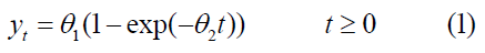
Because θ1,θ2>0 represent the model parameters and the value of yt changes with the change in the value of t, if t=∞ then yt =0 and when t→∞ means yt =θ1. To clarify the shape of the function, the first and second derivatives of Eq (1) are as follows:
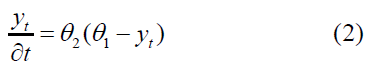
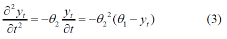
We note that the second derivative is less than zero and closer. t=∞ is to yt=θ1, The slope of the function is positive and increasing. By dividing equation (2) by yt, We obtain:
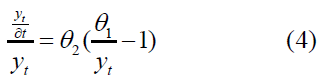
Thus, the rate of the new value at time t approaches zero when t→∞. To estimate the parameters of the Negative Exponential model, we take the natural logarithm of Eq (1) and obtain the following equation [3].
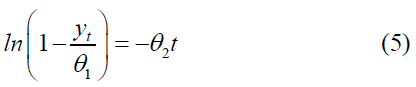
After determining the initial estimate of the -parameter θ1, denoted by θ*1The above equation can be written as follows:
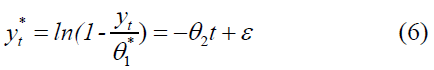
By solving the above equation, we obtain the parameter's initial value. θ2, denoted by θ2*.
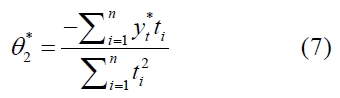
The initial estimates of the two parameters (θ1*, θ2*), in the first steps of Gauss-Newton. To achieve the best estimators and minimize the sum of squared errors 
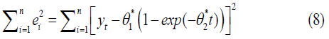
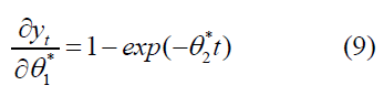
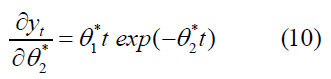
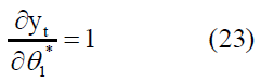
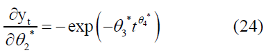
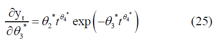
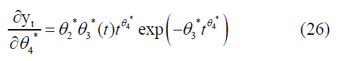
The partial derivatives of the parameters were:
Weibull Model
The Weibull model can be expressed in the following form:
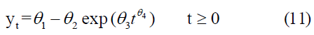
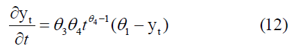
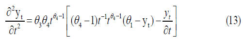
Since theta sub1, theta sub2, theta sub3,4, represent model parameters and take positive values , the value of t changes with the change in the value of tIf t=0, When it goes to infinity, it means y sub t goes to theta sub-1. To clarify the shape of the function, the first and second derivatives of Eq (11) are obtained as follows [4,12].
From the second derivative, when 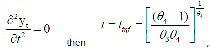 , by substituting the value of t in equation No. (11), we get:
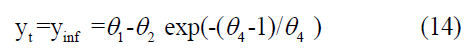
Thus, the inflection point of the Weibull function is (tinf, yinf) , Dividing equation (8) by yt, we obtain [5,13].
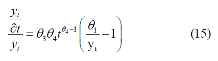
The growth rate of a new value at the time t approaches zero as t→∞approaches. From Eq (15), we obtain.
Starting Values of Parameters of Weibull Model
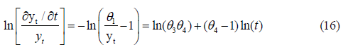
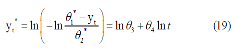
We used the natural logarithm twice for the equation to estimate the parameters of the Weibull model Eq. (11). The following equation is obtained [13-16]:
The initial estimate of the parameter θ1, denoted by θ1*, can be determined at the minimum value of t and the value of the parameter θ2* is determined from the following formula:
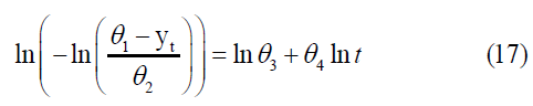
Where yinf represents the value of the coordinate of the constant term when t=0, and equation (17) can be expressed as follows:
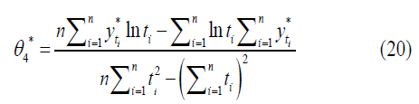
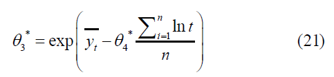
Using the least-squares method (LS) of (19), the initial estimates of the two parameters θ3, θ4, denoted by θ3*,θ4* and can be obtained as follows:
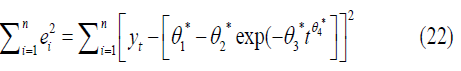
Using the values of the initial estimates of the parameters (θ1*, θ2*, θ3*, θ4*), the first steps of Gauss-Newton to achieve the best estimators and make the sum of the squares of the errors  the least possible, that is
Methods to Estimate the Parameter of Nonlinear Models
Nonlinear regression models are complicated and interrelated, and the estimation of their parameters is complex. There are several estimation methods, and we will discuss them below.
Nonlinear Least Square Method
The nonlinear least-squares method is one of the most essential and simplest methods for nonlinear regression analysis. We assume that we have a nonlinear model [17-19]:
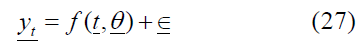
Since
Where:
yt: The vector represents the response values.
f: represents the function of ti, θ.
∈i: represents a random error that is normally distributed with zero mean μ and constant variance σ2 for all values of i. By using the nonlinear least-squares method, the following amount can be minimized:
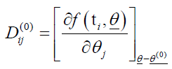
Using the Gauss-Newton method, θ_0=(θ10,θ20,…,θp0 )/. The initial values of the parameters are represented, and after approximating this series using the Taylor series expansion by eliminating the terms containing the partial derivatives of the higher degree, we obtain [8].
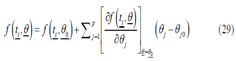
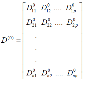
Where  initial values represent
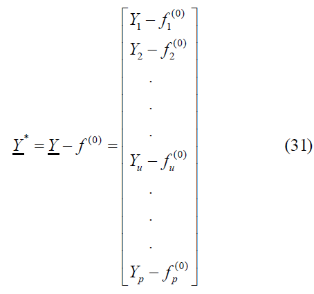
  if:
if:
So,
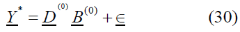
The parameters can then be estimated.  , or the equation (30) is using the ordinary least squares method through the following formula:
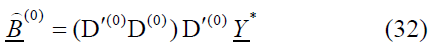

The estimated values for B(0) be:
From equation (33), we can obtain the value of  represents the modified estimated values of
  at the first iteration
  and is placed instead of the initial estimated value
  , and so on. The modified estimates can be rewritten as a-vectors in the following form:
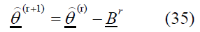
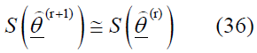
The iterations continue until convergence is reached between the two successive estimates (r) and (r + 1), such that:
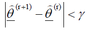
Since γ represents the minimal value. Note that S(θ), or each cycle of repetition and stopping according to the following formula:
Mathematical Equations of Criteria for Model Selection
When dealing with several models, the question is how to select the best from the competing models. Depending on the model structure, many statistical criteria can be used to choose the most appropriate model, such as [20-23]:
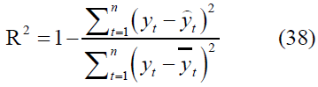
• Adjusted coefficient of determination, 
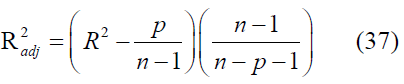
Where
• F-test
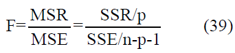
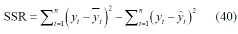
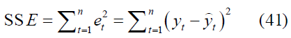
Where SSR is the sum squared of regression, and SSE is the sum squared of residuals (error), such that:
• Akaike Information Criterion (AIC)
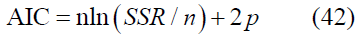
• Bayesian Information Criterion (BIC)
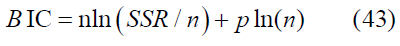
For AIC and BIC criteria, a smaller value indicates a preferable model.
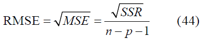
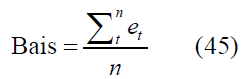
Goodness of Fit Criteria for Model
These indicate how well the model fits the actual data, with small residual values indicating a model fit. The most commonly used criteria are Mean Squared Error (MSE), Root Mean Squared Error (RMSE), and Mean Absolute error (MAE). These values are calculated as follows [24,25]:
Data
The study data represents the quarterly time series of cumulative maternal mortality, as collected from the Ministry of Health and Social Development - Statistics and Information Office - Red Sea State in Port Sudan, based on data from maternal mortality records for 2017-2023, as shown in Tab. 1.
| Date | Maternal Mortality |
|---|---|
| 2017(Q1) | 71 |
| 2017(Q2) | 120 |
| 2017(Q3) | 142 |
| 2017(Q4) | 243 |
| 2018(Q1) | 247 |
| 2018(Q2) | 328 |
| 2018(Q3) | 370 |
| 2018(Q4) | 399 |
| 2019(Q1) | 408 |
| 2019(Q2) | 502 |
| 2019(Q3) | 596 |
| 2019(Q4) | 662 |
| 2020(Q1) | 735 |
| 2020(Q2) | 748 |
| 2020(Q3) | 752 |
| 2020(Q4) | 815 |
| 2021(Q1) | 878 |
| 2021(Q2) | 937 |
| 2021(Q3) | 11001 |
| 2021(Q4) | 11030 |
| 2022(Q1) | 11038 |
| 2022(Q2) | 11123 |
| 2022(Q3) | 11206 |
| 2022(Q4) | 11260 |
| 2023(Q1) | 11388 |
| 2023(Q2) | 11446 |
| 2023(Q3) | 11462 |
| 2023(Q4) | 11632 |
Tab. 1. The cumulative number of maternal mortality cases in Red Sea State 2017-2023.
Fig. 1. shows the growth curve of maternal mortality over the study period, similar to S.

Fig. 1. The cumulative number mean fetal heart rate of time.
Results and Discussion
Starting Values of Parameters
For the Negative Exponential model, as explained above, we choose θ1 as the maximum cumulative maternal mortality cases, so  , and the estimation of eq (6) yields
  .
.
For the Weibull model, we choose θ1 is chosen as in the other models,  , and the estimation of eq (16) yields
 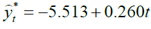 , so
, so 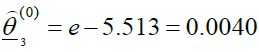 and
and  (Tab. 2.).
| Negative Exponential | Weibull | |
|---|---|---|
| Parameter | θ1 θ2 | θ1 θ2 θ3 θ3 |
| Initial | 11798 0.163 | 11798 11798 0.0040 1.260 |
Tab. 2. Starting values for studied growth models.
Estimation of Parameters of Nonlinear Models (Fig. 2.)

Fig. 2. Fitting growth models to the cumulative number of maternal mortalities.
Negative exponential estimated model:

Weibull estimated model:

Tab. 3. shows estimated parameters, standard errors, and 95% confidence lower and upper intervals.
| Model | Parameter | Estimator | Std. Error | 95% Confidence Interval | |
|---|---|---|---|---|---|
| Lower Bound | Upper Bound | ||||
| Neg.Exp. | θ1 | 5957931.01 | 3.548E+09 | -7.288E+09 | 7.3E+09 |
| θ2 | 0.00006 | 0.038 | -0.079 | 0.079 | |
| Weibull | θ1 | 1063525.777 | 7.516E+12 | 1.551E+13 | 1.551E+13 |
| θ2 | 1078503.149 | 7.516E+12 | 1.551E+13 | 1.551E+13 | |
| θ3 | 462822.098 | 1943737.6 | 3548855.2 | 4474499.4 | |
| θ4 | 4.511 | 1.894 | -8.42 | -0.602 | |
Tab. 3. Estimated results of the growth models under study.
The fitted Weibull model's parameter estimations are statistically significant at the 5% level, as the confidence intervals of all model estimators exclude zero. The estimation of several parameters in the Negative Exponential model is insignificant. This indicates that the Weibull model may better fit other models for describing the number of maternal mortality cases in the Red Sea station.
Model Selection Criteria
Tab. 4. shows the variance analysis results for the two models. The F-ratio values show that both models are statistically significant at the α = 1% level. When comparing the results of the two models, the Weibull model has the highest F-ratio, indicating that it was selected over the data.
| Model | Source | Sum of Squares | df | Mean Squares | F-ratio | P-value |
|---|---|---|---|---|---|---|
| Neg.Exp | Regression | 988514631.933 | 2 | 494257315.966 | 45.06** | 0.000 |
| Residual | 285220793.067 | 26 | 10970030.503 | |||
| Weibull | Regression | 1242874280.859 | 4 | 310718570.215 | 241.639** | 0.000 |
| Residual | 30861144.141 | 24 | 1285881.006 | |||
| Uncorrected Total | 1273735425.000 | 28 | ||||
| Corrected Total | 746173692.107 | 27 | ||||
| ** statistically significant at 1% level | ||||||
Tab. 4. ANOVA results for the growth models under study.
Tab. 5. shows additional criteria, including  , AIC and BIC support the above result. The Negative Exponential models evaluated had . The value is smaller, 0.538, with the Weibull model having the most outstanding value, 0.785, compared to the Negative Exponential model. According to AIC and BIC, the Weibull model has the lowest values of AIC 490.63 and 499.70 compared to the Negative Exponential model.
| Criteria | Neg.Exp | Weibull |
|---|---|---|
| RMSE | 3312.10 | 1133.97 |
| Bias | 843.98 | 0.7423 |
| MAE | 2884.76 | 528.72 |
| R2 | 0.618 | 0.959 |
| R2adj | 0.538 | 0.785 |
| AIC | 501.04 | 490.63 |
| BIC | 506.37 | 493.21 |
Tab. 5. Results of criteria and goodness of fit for the growth models under study.
Goodness of Fit
Tab. 5. shows that the Weibull model provides the most excellent fit, with the lowest RMSE, 1133.97, compared to the Negative Exponential model. On the other hand, the Weibull model had the lowest bias value, 0.7423, and the smallest MAE value, 528.72. The Weibull model's projected maternal mortality cases closely match the cumulative cases.
Forecasting
Maternal mortality is typically accompanied by several random variables that cannot be measured or controlled. Thus, forecasting the number of maternal mortalities will not be completely accurate and will not provide the same real numbers; the model will only estimate the number of maternal deaths. Table 6 and Figure 3 illustrate the quarterly cumulative confirmed maternal mortality in the Red Sea State using the Weibull growth model. We expect that the number of maternal mortalities in the Red Sea State will rise at a rate ranging from 10904.4 to 134360 cases over the next four years (2024-2026). Thus, this will provide reference information for competent authorities (Fig. 3. and Tab. 6.).

Fig. 3. Forecasts of cumulative maternal mortality cases by the Weibull model.
| t | Date | Forecasts | 95% CI |
|---|---|---|---|
| 30 | 2024(Q1) | 17231.6 | (10904.4; 23559) |
| 31 | 2024(Q2) | 18702.3 | (11577.4; 25827) |
| 32 | 2024(Q3) | 20251.6 | (10361.4; 30142) |
| 33 | 2024(Q4) | 21881.4 | (9560.7; 34202) |
| 34 | 2025(Q1) | 23593.7 | (8098.5; 39089) |
| 35 | 2025(Q2) | 25390.5 | (7750.3; 43031) |
| 36 | 2025(Q3) | 27273.9 | (5446.1; 49102) |
| 37 | 2025(Q4) | 29245.7 | (2064.9; 56427) |
| 38 | 2026(Q1) | 31308.2 | (1478.5; 64095) |
| 39 | 2026(Q2) | 33463.2 | (2164.9; 69091) |
| 40 | 2026(Q3) | 35712.9 | (7804.4; 79230) |
| 41 | 2026(Q4) | 38059.3 | (12953.3; 89072) |
| 42 | 2027(Q1) | 40504.5 | (18448.2; 99457) |
| 43 | 2027(Q2) | 43050.5 | (23932.2; 110033) |
| 44 | 2027(Q3) | 45699.5 | (29545.6; 120945) |
| 45 | 2027(Q4) | 48453.5 | (37452.7; 134360) |
Tab. 6. Forecasts of maternal mortality cases from the Weibull model.
To interpret the inflection point of the Weibull model, which was the best fit for the present data than the negative binomial model, apply Equation 14 to get: (tinf.,ŷinf.)=(34, 23593.7). The time index (t=34) gives the inflection point position when the growth rate is at its maximum. At this time, the maximum growth rate is (23593.7).
Conclusion
This study assessed Weibull and negative binomial models in comparison to the maternal mortality models of the Red Sea State. The Weibull model effectively depicted the maternal mortality curve in the Red Sea State. The goodness-of-fit criteria were evaluated to choose the ideal model representing the curve for the quarterly cumulative cases of maternal death. The conclusion was that the Weibull model produced the most favorable outcomes. The value was 0.785, the minimum bias value was 0.7423, the lowest RMSE was 1133.97, and the AIC was 490.63, in comparison to the Negative Binomial model. Consequently, the quarterly total of maternal fatalities in the Red Sea State may reach 48,453.5 after four years (2027 Q4), with a 95% confidence range ranging from 37,452.7 to 134,360. The current research models and some metrics were estimated using the "Nonlinear Regression" tool in Minitab-17, using the nonlinear least squares approach and calculating the starting values of the model parameters by the basic linear regression equation.
Prospective Studies
This study offers a significant comparison between the negative exponential model and the Weibull model for cumulative maternal mortality; however, subsequent research could employ fractional ordering models, as recent studies indicate that fractional models afford enhanced flexibility in depicting memory effects in epidemiological data, whereas conventional growth models depend on integer ordering dynamics [26-29].
Future studies may use fractional mathematical modelling to analyses the impact of long-term memory on maternal mortality trends. The lack of diverse intervention options significantly constrains our research. Guma, et al. [30] shown that mathematical modelling helps assess infectious disease management strategies. Employing this approach for maternal mortality assessment may enhance the evaluation of initiatives designed to improve prenatal care, mother health education, and emergency response systems.
Future study should investigate stochastic changes in maternal mortality to include exogenous shocks, such as epidemics and natural disasters, along with inaccuracies in the reporting of maternal deaths, as shown by Ali, et al. [31-34].
Acknowledgment
The author expresses his gratitude to the Statistics Department, Ministry of Health - Red Sea State, Sudan.
Declaration of Competing Interest
The author declares that they have no known competing financial Interests or personal relationships that could have appeared to influence the work reported in this paper.
Conflicts of Interest
The author declares no conflicts of interest regarding the publication of this paper.
References
- Midhet F, Khalid SN, Baqai S, et al. Trends in the levels, causes, and risk factors of maternal mortality in Pakistan: A comparative analysis of national surveys of 2007 and 2019. PLoS One. 2025;20(1):e0311730.
- Poletto JP. An alternative to the exponential and Weibull reliability models. IEEE Access. 2022;10:118759-78.
- Gupta RD, Kundu D. Discriminating between Weibull and generalized exponential distributions. Comput Stat Data Anal. 2003;43(2):179-96.
- S Alduais F, Khan Z. Development of Neutrosophic Gamma Distribution for Modeling Neonatal Mortality Data. Neutrosophic Sets Syst. 2025;79(1):48.
- Shakir GH, Hassan I. Study of new Exponential-Weibull distribution about children with Leukemia. INAIP Conf Proc. AIP Publishing. 2024 ; 3036( 1).
- Aliyu S, Bamanga MA. Estimation and comparison of Weibull-Normal distribution with some other probability models using Bayesian method of estimation. Sci World J. 2024;19(1):92-100.
- Imran M, Alsadat N, Tahir MH, et al. The development of an extended Weibull model with applications to medicine, industry and actuarial sciences. Sci Rep. 2024;14(1):12338.
- Sharma P, Gupta BM, Kumar S. Application of growth models to science and technology literature in research specialities. DESIDOC J Lib Infor Tech. 2002;22(2).
- Lee PN, Hamling J, Fry J, et al. Using the negative exponential model to describe changes in risk of smoking-related diseases following changes in exposure to tobacco. Adv Epidemiol. 2015;2015(1):487876.
- Aryuyuen S, Bodhisuwan W. The negative binomial-generalized exponential (NB-GE) distribution. Appl Math Sci. 2013;7(22):1093-105.
- Myers RH, Montgomery DC, Vining GG, et al. Generalized linear models: with applications in engineering and the sciences. John Wiley & Sons; 2012.
- Lai CD, Murthy DN, Xie M. Weibull distributions. Wiley Interdiscip Rev Comput Stat. 2011;3(3):282-7.
- Teimouri M, Hoseini SM, Nadarajah S. Comparison of estimation methods for the Weibull distribution. Statistics. 2013;47(1):93-109.
- Alshanbari HM, Ahmad Z, El-Bagoury AA, et al. A new modification of the Weibull distribution: Model, theory, and analyzing engineering data sets. Symmetry. 2024;16(5):611.
- Al Zahrani S, Al Sameeh FA, Musa AC, et al. Forecasting diabetes patients attendance at al-baha hospitals using autoregressive fractional integrated moving average (arfima) models. J Data Anal Infor Process. 2020;8(03):183.
- Mahanta DJ, Borah M. Parameter estimation of Weibull growth models in forestry. Int J Math Trends Tech. 2014;8.
- Mohiuddin AM, Bansal JC. An improved linear prediction evolution algorithm based on nonlinear least square fitting model for optimization. Soft Comput. 2023;27(19):14019-44.
- Draper NR, Smith H. Applied regression analysis. John Wiley & Sons; 1998.
- Guma FE, Badawy OM, Musa AG, et al. Risk factors for death among COVID-19 Patients admitted to isolation Units in Gedaref state, Eastern Sudan: a retrospective cohort study. J Surv Fish. 2023;10(3s):712-22.
- Bezerra AK, Santos ÉM. Prediction the daily number of confirmed cases of COVID-19 in Sudan with ARIMA and Holt Winter exponential smoothing. Int J Dev Res. 2020;10(08):39408-13.
- Ghanim Al-Ani B. Statistical modeling of the novel COVID-19 epidemic in Iraq. Epidemiol Methods. 2021;10(s1):20200025.
- Gratton S, Lawless AS, Nichols NK. Approximate Gauss–Newton methods for nonlinear least squares problems. SIAM J Optim. 2007;18(1):106-32.
- Shokeralla AA, Qurashi ME, Mekki RY, et al. The Effect of Symptoms on the Survival Time of Coronavirus Patients in the Sudanese Population.
- Alzahrani SM, Guma FE. Improving Seasonal Influenza Forecasting Using Time Series Machine Learning Techniques. J Inf Syst Eng Manag. 2024;9(4):30195.
- Fath-Elrhman EI, Abdelaziz GM, Shokeralla AA, et al. Modeling sudan’s inflation rate using multilayer feed forward neural network with back propagation algorithm. Int J Eng Sci Math. 2020;9(10):1-1.
- Saadeh R, Abdoon MA, Qazza A, et al. Mathematical modeling and stability analysis of the novel fractional model in the Caputo derivative operator: A case study. Heliyon. 2024;10(5).
- Abdulkream Alharbi S, A. Abdoon M, Saadeh R, et al. Modeling and analysis of visceral leishmaniasis dynamics using fractional-order operators: A comparative study. Math Methods Appl Sci. 2024;47(12):9918-37.
- E. Alsubaie N, EL Guma F, Boulehmi K, et al. Improving influenza epidemiological models under Caputo fractional-order calculus. Symmetry. 2024;16(7):929.
- Alharbi SA, Abdoon MA, Degoot AM, et al. Mathematical modeling of influenza dynamics: A novel approach with SVEIHR and fractional calculus. Int J Biomath. 2025:2450147.
- Gumaa FE, Abdoon MA, Qazza A, et al. Analyzing the impact of control strategies on VisceralLeishmaniasis: a mathematical modeling perspective. Eur J Pure Appl. 2024;17(2):1213-27.
- Ali M, Guma FE, Qazza A, et al. Stochastic modeling of influenza transmission: Insights into disease dynamics and epidemic management. Partial Differ Equ Appl Math. 2024;11:100886.
- Ali M, Alzahrani SM, Saadeh R, et al. Modeling COVID-19 spread and non-pharmaceutical interventions in South Africa: A stochastic approach. Sci African. 2024;24:e02155.
- Hung HF, Wang YC, Yen AM, et al. Stochastic model for hepatitis B virus infection through maternal (vertical) and environmental (horizontal) transmission with applications to basic reproductive number estimation and economic appraisal of preventive strategies. Stoch Env Res Risk A. 2014;28:611-25.
- Bakari HR, Mustapha M, Ladan FB. Statistical Analysis of Human Fertility Behavior Using Probability Distributions. Int J Math Oper Res. 2018;14(3):77-85.
Google Scholar, Cross Ref, Indexed at
Google Scholar, Cross Ref, Indexed at
Google Scholar, Cross Ref, Indexed at
Google Scholar, Cross Ref, Indexed at
Google Scholar, Cross Ref, Indexed at
Google Scholar, Cross Ref, Indexed at
Google Scholar, Cross Ref, Indexed at
Google Scholar, Cross Ref, Indexed at
Google Scholar, Cross Ref, Indexed at
Google Scholar, Cross Ref, Indexed at
Google Scholar, Cross Ref, Indexed at
Google Scholar, Cross Ref, Indexed at
Google Scholar, Cross Ref, Indexed at
Google Scholar, Cross Ref, Indexed at
Google Scholar, Cross Ref, Indexed at
Google Scholar, Cross Ref, Indexed at
Google Scholar, Cross Ref, Indexed at
Google Scholar, Cross Ref, Indexed at
Google Scholar, Cross Ref, Indexed at
Google Scholar, Cross Ref, Indexed at
Author Info
Alshaikh A. Shokeralla*Copyright:This is an open access article distributed under the terms of the Creative Commons Attribution License, which permits unrestricted use, distribution, and reproduction in any medium, provided the original work is properly cited.